Using the python backend

Here we illustrate some ways of using pymagglobal from within python. For explicit documentation, see here.

Creating a Model instance

The first step to work with pymagglobal models is to make them accessible by instancing the Model class. We therefore import Model and create an instance by passing the name of the model we want to access, in this case GGFMB:

from pymagglobal import Model

ggfmb = Model('GGFMB')

We can access some information about the model, for example the maximum degree:

print(ggfmb.l_max)

6

We can also use the valid_epoch method to check if an epoch is covered by the model:

# pass the epoch as yr.

ggfmb.valid_epoch(-700_000)

array(-700000)

valid_epoch returns the input, but throws a warning if the input is not covered by the model:

# pass the epoch as yr.

ggfmb.valid_epoch(-2_000)

/opt/conda/envs/deploying/lib/python3.11/site-packages/pymagglobal/core.py:179: OutOfRangeWarning: Epochs [-2000] are outside of the models range [-898050.0, -698050.0]. The result will be extrapolated and not robust.

array(-2000)

Using core functions

The most straight-forward way of extracting specific information from a model is to use the core functions of pymagglobal. Check the documentation to see which functions are available.

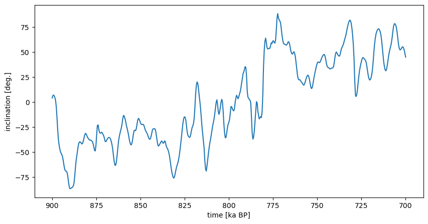
Let’s assume we want to get a local time series of the inclination at a specific location. We can use the local_curve function for that:

import numpy as np

from pymagglobal import local_curve

# Honululu as lat, lon tuple
loc = (21.306944, -157.858333)

# Create an evenly spaced array over the ggfmb interval

times = np.linspace(
    ggfmb.t_min,
    ggfmb.t_max,
    501,
)
d, i, f = local_curve(times, loc, ggfmb)

We can now plot the result. Note that we convert the input to kiloyears before present for better readability:

from matplotlib import pyplot as plt

from pymagglobal.utils import yr2lt

fig, ax = plt.subplots(1, 1, figsize=(10, 5))

ax.plot(
    yr2lt(times),
    i,
)
ax.invert_xaxis()
ax.set_xlabel('time [ka BP]')
ax.set_ylabel('inclination [deg.]');

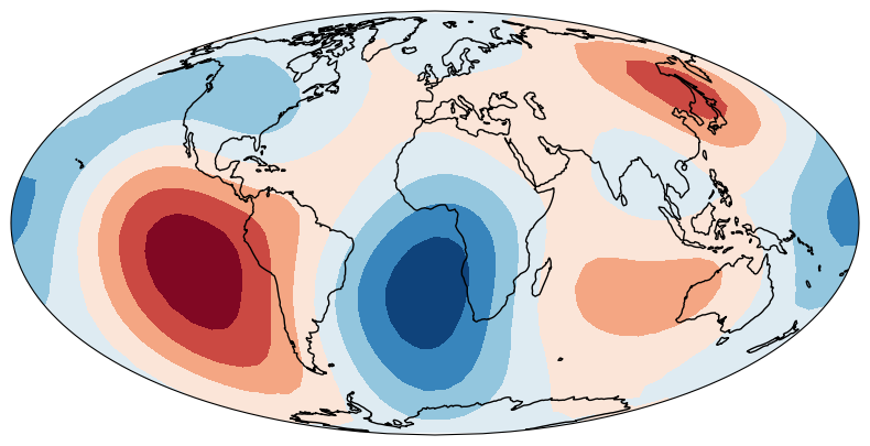
We might also be interested in a map of the radial component (Z) of the field at the Earth’s surface. We can use the field method to create such a map:

from pymagglobal import field
from pymagglobal.utils import get_grid, lt2yr

# Set up a grid at the Earth's surface
# The epoch 780 ka BP is transformed to years using lt2yr
grid = get_grid(1000, t=lt2yr(780))
# for plotting purposes shift the array
grid[1] -= 180
# access is then straight-forward
n, e, z = field(grid, ggfmb)

We can plot the result using cartopy:

from cartopy import crs as ccrs

proj = ccrs.Mollweide()

fig, ax = plt.subplots(1, 1, figsize=(10, 5), subplot_kw={'projection': proj})

plt_lat, plt_lon, _ = proj.transform_points(
    ccrs.Geodetic(),
    grid[1],
    90-grid[0],
).T

vmax = np.max(np.abs(z))
ax.tricontourf(
    plt_lat,
    plt_lon,
    z,
    vmax=vmax,
    vmin=-vmax,
    cmap='RdBu',
)
ax.set_global()
ax.coastlines();

/opt/conda/envs/deploying/lib/python3.11/site-packages/cartopy/io/__init__.py:241: DownloadWarning: Downloading: https://naturalearth.s3.amazonaws.com/110m_physical/ne_110m_coastline.zip

Using model coefficients directly

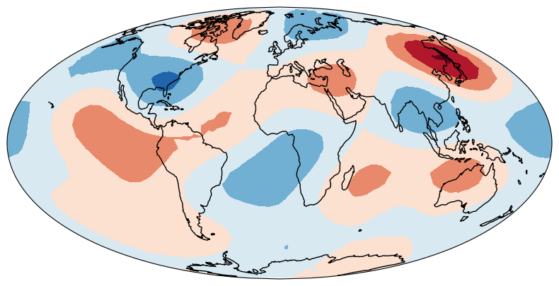
If we are intersted in something that is not available directly via the core functions, we might be able to use model coefficients directly and calculate the quantity of interst. Here we show how to generate a map of the radial (Z) component of the field at the core-mantle boundary. There are two ways to do this. Either we scale the coefficients and use unscaled basis functions, or we might also have the basis functions include a scaling. To highlight several aspects of pymagglobal we pursue the first approach. Initially, we access the coefficients for the specific epoch at the Earth’s surface:

from pymagglobal import coefficients

l, m, coeffs = coefficients(lt2yr(780), ggfmb)

Next we scale the coeffients to the core-mantle boundary (3480 km):

from pymagglobal.utils import scaling, REARTH

coeffs_cmb = coeffs * scaling(REARTH, 3480, ggfmb.l_max)

In order to calculate the field components, we evaluate the basis functions at the grid specified before. The basis functions are derivatives of the spherical harmonics. The function dsh_basis takes array of shape (L, 3*N), where L is the number of Gauss coefficients, as third argument and fills it with the appropriate values. We calculate the number of coeffients from the maximum spherical harmonics degree using lmax2N. Note that by default, dsh_basis assumes that the coefficients are given at the Earth’s surface. I.e. if the grid is also at the Earth’s surface, no scaling is applied. If however the radial grid entries grid[2] differ from REARTH, dsh_basis automatically includes a scaling. Check the end of this notebook for the way to handle this scalings explicitly.

from pymagglobal.utils import dsh_basis, lmax2N

base = np.empty((lmax2N(ggfmb.l_max), 3*grid.shape[1]))
dsh_basis(ggfmb.l_max, grid, base)

array([[-5.60704472e-02,  0.00000000e+00, -1.99685363e+00, ...,
        -5.60704472e-02,  0.00000000e+00,  1.99685363e+00],
       [-9.98426815e-01, -1.22464680e-16,  1.12140894e-01, ...,
         9.98426815e-01,  1.22464680e-16,  1.12140894e-01],
       [-1.83408030e-16,  1.00000000e+00,  2.05999481e-17, ...,
        -6.11360102e-17,  1.00000000e+00, -6.86664937e-18],
       ...,
       [-2.80657566e-19,  1.14811120e-04,  2.20798743e-20, ...,
         6.31319979e-20, -1.14811120e-04,  4.96671655e-21],
       [ 2.23001917e-06,  1.64117338e-21, -1.46107722e-07, ...,
        -2.23001917e-06, -1.64117338e-21, -1.46107722e-07],
       [-2.18616901e-21, -2.23353293e-06,  1.43234721e-22, ...,
         5.46335203e-21, -2.23353293e-06,  3.57951147e-22]])

Calculating the field is then straight forward, we simply multiply the coefficients and the basis:

nez_cmb = coeffs_cmb @ base

To access the radial component we reshape the field array:

nez_cmb = nez_cmb.reshape(grid.shape[1], 3).T
z_cmb = nez_cmb[2]

We can again plot the results using cartopy:

fig, ax = plt.subplots(1, 1, figsize=(10, 5), subplot_kw={'projection': proj})

vmax = np.max(np.abs(z_cmb))
ax.tricontourf(
    plt_lat,
    plt_lon,
    z_cmb,
    vmax=vmax,
    vmin=-vmax,
    cmap='RdBu',
)
ax.set_global()
ax.coastlines();

In this case we could have also set the radius of the grid to the core-mantle boundary and use the field routine. This implicitly moves the scaling to the basis functions as mentioned above:

grid_cmb = np.copy(grid)
grid_cmb[2] = 3480

_, _, z_cmb_2 = field(grid_cmb, ggfmb)

fig, ax = plt.subplots(1, 1, figsize=(10, 5), subplot_kw={'projection': proj})

ax.tricontourf(
    plt_lat,
    plt_lon,
    z_cmb_2,
    vmax=vmax,
    vmin=-vmax,
    cmap='RdBu',
)
ax.set_global()
ax.coastlines();

The formally correct/explicit way of using dsh_basis like above would be to both move the grid to the core-mantle boundary and use dsh_basis with 3480 km as reference radius like so:

base_cmb = np.empty((lmax2N(ggfmb.l_max), 3*grid_cmb.shape[1]))
dsh_basis(ggfmb.l_max, grid_cmb, base_cmb, R=3480)

nez_cmb_3 = coeffs_cmb @ base_cmb
nez_cmb_3 = nez_cmb_3.reshape(grid.shape[1], 3).T
z_cmb_3 = nez_cmb_3[2]

fig, ax = plt.subplots(1, 1, figsize=(10, 5), subplot_kw={'projection': proj})

ax.tricontourf(
    plt_lat,
    plt_lon,
    z_cmb_3,
    vmax=vmax,
    vmin=-vmax,
    cmap='RdBu',
)
ax.set_global()
ax.coastlines();

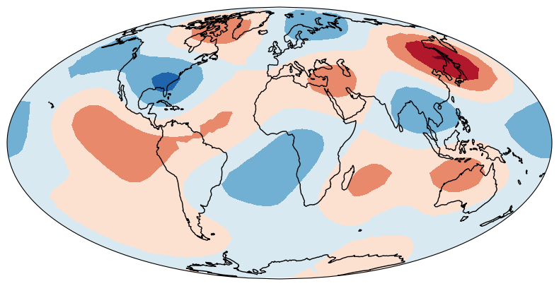
Due to the implicit scaling applied above, base_cmb and base are actually identical:

assert(np.all(base == base_cmb))