Generate synthetic data

Here we briefly show how pymagglobal can be used to generate synthetic data. We first set up the model we want to use to generate the synthetic data:

from pymagglobal import Model

myModel = Model('CALS10k.2')

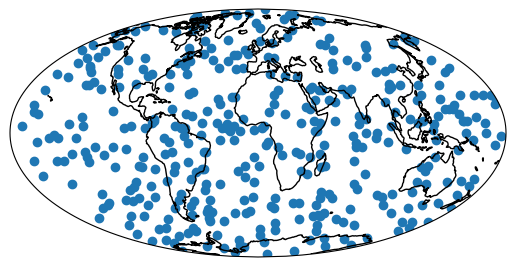
Next we have to generate a data distribution. We use pymagglobals get_grid routine, to generate n_at random locations, that are uniformly distributed on the sphere. Times are drawn uniformly as well.

from pymagglobal.utils import get_grid

import numpy as np
from matplotlib import pyplot as plt
from cartopy import crs as ccrs

# the number of artificial records
n_at = 400
grid = get_grid(n_at, random=True)
# set the times to something arbitrary
grid[3] = np.random.uniform(-1000, 1900, size=n_at)

# plot the records, convert colat to lat
fig, ax = plt.subplots(1, 1, subplot_kw={'projection': ccrs.Mollweide()})
ax.scatter(grid[1], 90-grid[0], transform=ccrs.PlateCarree())
ax.set_global()
ax.coastlines();

Finally we can evaluate the model at the inputs, to get synthetic ‘’observations’’ of the field

from pymagglobal.core import field
obs = field(grid, myModel)

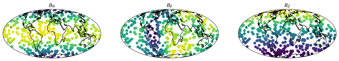
Let’s have a look at the records:

fig, axs = plt.subplots(1, 3, subplot_kw={'projection': ccrs.Mollweide()},
                        figsize=(15, 4))
titles = [r'$B_N$', r'$B_E$', r'$B_Z$']
for it in range(3):
    axs[it].set_title(titles[it])
    axs[it].scatter(
        grid[1],
        90 - grid[0],
        c=obs[it], transform=ccrs.PlateCarree(),
    )
    axs[it].set_global()
    axs[it].coastlines();

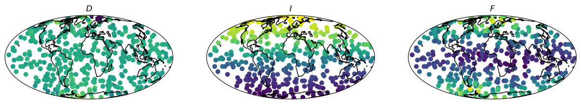
Declination, inclination and intensity records are also easily generated, by using the field kwargs:

obs_dif = field(grid, myModel, field_type='dif')
fig, axs = plt.subplots(1, 3, subplot_kw={'projection': ccrs.Mollweide()},
                        figsize=(15, 4))
titles = [r'$D$', r'$I$', r'$F$']
for it in range(3):
    axs[it].set_title(titles[it])
    axs[it].scatter(grid[1], 90-grid[0], c=obs_dif[it], transform=ccrs.PlateCarree())
    axs[it].set_global()
    axs[it].coastlines();

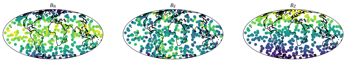
Data from an arbitray set of coefficients

Sometimes it is helpful to generate data not from a model that’s included in pymagglobal, but from an arbitrary set of coefficients. Provided they are in the ‘’standard order’’, i.e. \(g_1^0, g_1^1, g_1^{-1}, g_2^0, g_2^1, g_2^{-1}, ...\), this is also straight-forward using utility routines from pymagglobal:

from pymagglobal.core import coefficients

epoch = -3000
# First generate coefficients at epoch
_, _, coeffs = coefficients(epoch, myModel)

# Generate new input locations at the given epoch
grid = get_grid(n_at, random=True, t=epoch)

We use the pymagglobal routine dsh_basis, which evaluates the derivatives of the spherical harmonics up to a given degree at given inputs:

from pymagglobal.utils import dsh_basis

base = dsh_basis(myModel.l_max, grid)

Field values are then generated via a dot product:

obs = coeffs @ base

The outputs are now given by obs, every third value is N, E, Z. To have a more convenient form, we reshape the output:

obs = obs.reshape(n_at, 3).T

fig, axs = plt.subplots(1, 3, subplot_kw={'projection': ccrs.Mollweide()},
                        figsize=(15, 4))
titles = [r'$B_N$', r'$B_E$', r'$B_Z$']
for it in range(3):
    axs[it].set_title(titles[it])
    axs[it].scatter(grid[1], 90-grid[0], c=obs[it], transform=ccrs.PlateCarree())
    axs[it].set_global()
    axs[it].coastlines();